Subscribe to our YouYube channel and click on bell icon : https://www.youtube.com/c/SNBosePhysicsLearningCenter/
Question paper and Answer Key : Click on the link given below
Part- B (3.5 Marks)
Q.No: 21
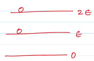
A part of an infinitely long wire, carrying a current \(I\), is bent in a semi-circular arc of radius \(r\) (as shown in the figure).

The magnetic field at the centre \(O\) of the arc is
(1)
\(\frac{\mu_0 I}{4r}\)
(2)
\(\frac{\mu_0 I}{4\pi r}\)
(3)
\(\frac{\mu_0 I}{2r}\)
(4)
\(\frac{\mu_0 I}{2\pi r}\)
Solution :
Magnetic field at 'O' due to straight line segment is zero.
Magnetic field at 'O' due to semi-circular arc is half the magnetic field due to circular ring
\[B_0=\frac{1}{2}\frac{\mu_0 I}{2r}=\frac{\mu_o I}{4r}\]
Answer : 1
Q.No: 22
The figure below shows a circuit with two transistors, \(Q_1\) and \(Q_2\) having current gain \(\beta_1\) and \(\beta_2\) respectively.

The collector voltage \(V_C\) will be closest to
(1)
\(0.9\) V
(2)
\(2.2\) V
(3)
\(2.9\) V
(4)
\(4.2\) V
Solution :
The circuit is called Darlington Pair

Referring to Boylestad 11th Edition, Chapter-4, Equations 4.50 to 4.53 :
\(\beta_D=\beta_1\times \beta_2=400\)
\(I_{c{_1}}=\beta_1 I_{B{_1}}\)
\(I_{B{_1}}=\frac{V_{cc}-V_{BE_1}-V_{BE_2}}{R_B+(\beta_D+1)R_E}=23.42\mu A\)
\(I_{c{_1}}=\beta_1 I_{B{_1}}=20\times 23.42\mu\)A = 0.446mA
\(I_{c{_2}}=\beta_D I_{B{_1}}=400\times 23.42\mu\)A = 9.36mA
So, \(I_c=I_{c{_1}}+I_{c{_2}}\), \(I_c=9.8\)mA
\(V_{cc}-I_c(1 k)-(V_c-0)=0\)
\(V_c=12-(9.8mA\times 1k\Omega)\)=2.2V
Answer : 2
Q.No: 23
If \(z=i^{i^{i^{.^{.}}}}\) (note that the exponent continuous indefinitely), then a possible value of \(\frac{1}{z}\) ln \(z\) is
(1)
2i ln i
(2)
ln i
(3)
i ln i
(4)
2 ln i
Solution :
\[z=i^{i^{i^{i^{.^{.}}}}}=i^{(i^{i^{i^{.^{.}}}})}\]
The term in the bracket is again and \(z\).
So, \(z=i^z\)
\(ln\hspace{1mm}z=z ln i\)
Therefore, value of \(\frac{1}{z}\hspace{1mm} ln z=ln\hspace{1mm} i\)
Answer : 2
Q.No: 24
If the expectation value of the momentum of a particle in one dimension is zero, then its (box-normalizable) wavefunction may be of the form
(1)
\(sin (kx) \)
(2)
\(e^{ikx} sin (kx) \)
(3)
\(e^{ikx}cos (kx) \)
(4)
\(sin (kx) + e^{ikx} cos (kx) \)
Solution :
\(\langle p\rangle =-i \hbar \int \psi^* \frac{\partial\psi}{\partial x} dx\)
\(\langle p\rangle\) should always be real. So \(\int \psi^* \frac{\partial\psi}{\partial x} dx\) is either purely imaginary or zero.
For real wave-function, if \(\int \psi^* \frac{\partial\psi}{\partial x} dx\) exists, then it will be real, which leads to imaginary \(\langle p\rangle\).
Therefore, for real wave-function, \(\int \psi^* \frac{\partial\psi}{\partial x} dx\) should vanish to make \(\langle p\rangle\) real.
Therefore, for a real wave-function :
\(\langle p\rangle=-i\hbar \int\psi^* \frac{\partial\psi}{\partial x} dx =0 \)
Only Option-1 contains real wave-function.
Q.No:27
Four students (\(S_1,S_2,S_3\) and \(S_4\)) make multiple measurements on the length of a table. The binned data are plotted as histograms in the following figures.

If the length of the table, specified by a manufacture, is 3m, the students whose measurements have the minimum systematic error, is
(1)
\(S_2\)
(2)
\(S_1\)
(3)
\(S_4\)
(4)
\(S_3\)
Solution :
The measured value should have least variance from actual value .
\(S_1\) have got the least variance (or standard deviation)
Q.No: 28
Two \(n\times n\) invertible real matrices A and B satisfy the relation
\((AB)^T=-(A^{-1}B)^{-1}\)
If B is orthogonal then A must be
(1)
lower triangle
(2)
orthogonal
(3)
symmetric
(4)
antisymmetric
Solution :
\((A \hspace{1mm}B)^T=-(A^{-1}\hspace{1mm}B)^{-1}\)
\(B\) is orthogonal \(\Rightarrow B^T=B^{-1}\)
\(B^T\hspace{1mm} A^T=-B^{-1}(A^{-1})^{-1}\)
\(B^{-1}\hspace{1mm}A^T=-B^{-1} A\)
\(A^T=-A\)
\(A\) is anti-symmetric
Q.No: 29
The Lagrangian of a system described by three generalized coordinates \(q_1,q_2\) and \(q_3\) is
\[L=\frac{1}{2}m(\dot{q}_1^2+\dot{q}_2^2)+M\dot{q}_1\dot{q}_2+k\dot{q}_1 q_3\]
where \(m,M\) and \(k\) are positive constants. Then, as a function of time
(4)
two coordinates remain constant and one evolves linearly
(4)
one coordinate remains constant, one evolves linearly and the third evolves as a quadratic function
(4)
one coordinate evolves linearly and two evolve quadratically
(4)
all three evolve linearly
Solution :
Lagrange's equation of motion are
\(q_1\) :
\(m\dot{q}_1+m\dot{q}_2+k\dot{q}_3=c_1\)---------------(1)
\(q_2\) :
\(m\dot{q}_2+m\dot{q}_1=c_2\) \(\Rightarrow m\frac{d}{dt}(q_1+q_2)=c_2\)
\(m(q_1+q_2)=c_2 t+ c'_2 \)-----------------------(2)
\(q_3\) :
\(k\dot{q}_1=0\) \(\Rightarrow q_1=c_4\) ---------------(3)
Subtracting (3) into (2) \(\Rightarrow q_2=ct+c'_1 \)----------(4)
Subtracting (3),(4) into (1) \(\Rightarrow q_3\) = constant. ---(5)
(Where \(c\) and \(c_i\) are constants)
So, \(q_1\) and \(q_3\) are constants and \(q_2\) varies linearly with respect to time.
Q.No: 30
The value of an integral \(\int_0^\infty dx\hspace{0.5mm} e^{-x^{2m}}\), where \(m\) is a positive integer, is
(1)
\(\Gamma (\frac{m+1}{2m})\)
(2)
\(\Gamma (\frac{m-1}{2m})\)
(3
)
\(\Gamma (\frac{2m+1}{2m})\)
(4)
\(\Gamma (\frac{2m-1}{2m})\)
Solution :
Let \(I=\int _0 ^\infty e^{-x^{2m}} dx \)
for \(m=1\),
\[I=\int _0 ^\infty e^{-x^{2}} dx =\frac{1}{2}\int _{-\infty} ^{+\infty} e^{-x^{2m}} dx =\frac{1}{2} \Gamma (\frac{1}{2})=\Gamma (\frac{3}{2})\]
Only option 3, \(\Gamma(\frac{2m+1}{2m})\) satisfy this.
Q.No:31 CSIR Sep-2022
Consider the Hamiltonian \(H=AI+B\sigma_x+C\sigma_y\), where \(A,B\) and \(C\) are positive constants, \(I\) is the \(2\times2\) matrix and \(\sigma_x\) and \(\sigma_y\) are Pouli matrices. If the normalized eigenvector corresponding to its largest energy eigenvelue is \(\frac{1}{\sqrt{2}}\begin{pmatrix} 1\\ y \end{pmatrix}\), then \(y\) is
(1)
\(\frac{B+iC}{\sqrt{B^2+C^2}}\)
(2)
\(\frac{A-iB}{\sqrt{A^2+B^2}}\)
(3)
\(\frac{A-iC}{\sqrt{A^2+C^2}}\)
(4
)
\(\frac{B-iC}{\sqrt{B^2+C^2}}\)
Solution :
\(H=AI+(B\hat{i}+C\hat{j})\cdot \vec{\sigma}\)
Eigenvalues of \((B\hat{i}+C\hat{j})\cdot \vec{\sigma}\) are \(\pm \sqrt{B^2+C^2}\)
he largest Eigenvalue of \(H\) is \(A+\sqrt{B^2+C^2}\)
\(H\frac{1}{\sqrt{2}}\begin{pmatrix} 1\\ y \end{pmatrix}=(A+\sqrt{B^2+C^2}) \frac{1}{\sqrt{2}} \begin{pmatrix} 1\\ y \end{pmatrix}\)
\(\left[ A\begin{pmatrix} 1&0\\ 0&1 \end{pmatrix} +B\begin{pmatrix} 0&1\\ 1&0 \end{pmatrix} +C \begin{pmatrix} 0& -i\\ i& 0 \end{pmatrix} \right] \begin{pmatrix} 1\\ y \end{pmatrix}\)
=\((A+\sqrt{B^2+C^2}) \begin{pmatrix} 1\\ y \end{pmatrix}\)
\(\Rightarrow \frac{\sqrt{B^2+C^2}}{B-iC}\times \frac{B+ iC}{B+ iC}=\frac{B+ iC}{\sqrt{B^2+C^2}}\)
Q.No:32 CSIR Sep-2022
At \(z=0\),the function \(\frac{1}{z- sin \hspace{1mm}z}\) of a complex variable \(z\) has
(1)
no singularity
(2)
a simple pole
(3)
a pole of order 2
(4)
a pole of order 3
Solution :
\(f(z)=\frac{1}{z-sin(z)}=\frac{1}{z-(z-\frac{z^3}{3!}+\frac{z^5}{5!}+.....)}\)
\(f(z)=\frac{1}{\frac{-z^3}{3!}+\frac{z^5}{5!}- ......}\)
\(\lim_{z \to 0}(z-0)^3 f(z)\) is non-zero and finite.
So, \(z=0\) is a pole of order 3
Q.No:34 CSIR Sep-2022
An elastic rod has a low energy state of length \(L_{max}\) and high energy state of length \(L_{min}\). The best schematic
representation of the temperature \((T)\) dependence of the mean equilibrium length \(L(T)\) of the rod, is

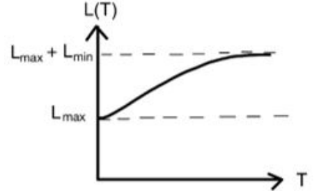


Solution :
\(E_1=C \hspace{2mm} L_{max}\) be the lowest energy.
\(E_2=C \hspace{2mm} L_{min}\) be the highest energy.
\(\langle L \rangle= L_{max} P(E_1) + L_{min} P(E_2)\)
\(P(E_1)=\frac{e^{-\beta E_1}}{e^{-\beta E_1}+e^{-\beta E_2}}\) , \(P(E_1)=\frac{e^{-\beta E_2}}{e^{-\beta E_1}+e^{-\beta E_2}}\)
As \(T \to \infty\) \(\beta \to 0 \) \(\frac{P(E_1)}{P(E_2)}=e^{-\beta(E_2-E_1)}\to 0\)
\(P(E_2)\approx 0\) \(\hspace{3mm}\) \(P(E_1)\approx 1\)
So, \(\langle L \rangle= L_{max}\)
As \(t \to \infty\) \(\beta \to \infty\) \(P(E_1)=P(E_2)\approx \frac{1}{2}\)
So, \(\langle L \rangle=(L_{max} + L_{min})/2\)

Q.No:35 CSIR Sep-2022
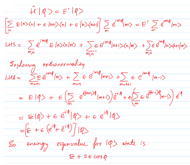
In terms of a complete set of orthonormal basis kets \(|n\rangle\), \(n=0,\pm 1, \pm 2,.....,\),the Hamiltonian is
\[H = \sum_n(E |n\rangle\langle n|\hspace{1mm} + \hspace{1mm}\epsilon |n+1\rangle \langle n|\hspace{1mm} +\hspace{1mm} \epsilon |n\rangle \langle n+1|)\]
where \(E\) and \(\epsilon\) are constants. The state \(|\varphi \rangle=\sum_n e^{in\varphi}|n\rangle\) is an eigenstate with energy
(1)
\(E + \hspace{1mm}\epsilon \hspace{1mm} cos \hspace{1mm} \varphi\)
(2)
\(E - \hspace{1mm}\epsilon \hspace{1mm} cos \hspace{1mm} \varphi\)
(3)
\(E + \hspace{1mm}2\epsilon \hspace{1mm} cos \hspace{1mm} \varphi\)
(4)
\(E - \hspace{1mm}2\epsilon \hspace{1mm} cos \hspace{1mm} \varphi\)
Solution :
Q.No:37 CSIR Sep-2022
Two positive and two negative charges of magnitude \(q\) are placed on the alternate vertices of a cube of side \(a\) (as shown in the figure)

The electric dipole moment of this charge configeration is
(1)
\(-2qa \hspace{1mm}\hat{k}\)
(2)
\(2qa \hspace{1mm}\hat{k}\)
(3)
\(2qa \hspace{1mm}(\hat{i}+\hat{j})\)
(4)
\(2qa \hspace{1mm}(\hat{i}-\hat{j})\)
Solution :
\(\vec{p}=\sum_i q_i \vec{r}\)
(\(\vec{r}\) is position vector of \(q_i\))
\(\vec{p}= +qa\hat{k}-qa\hat{j}-qa\hat{i}+qa(\hat{i}+\hat{j}+\hat{k}\))\
\(\vec{p}=2qa\hat{k}\)
Q.No:38 CSIR Sep-2022
A high impedance load (network) is connected in the circuit as shown below.

The forward voltage drop for silicon diode is 0.7 V and Zener voltage 9.10 V. If the input voltage \((V_{in})\) is sine wave with an amplitude of 15 V (as shown in the figure above) , which one of the following waveform qualitatively describes the output voltage \((V_{out})\) across the load ?


Solution :

In the second circuit case, Zener diode is in no-bias condition. For no-bias \(\Rightarrow I=0 , V=0\)

Q.No:39 CSIR Sep-2022
An electromagnetic wave is incident from vacuum normally on a planar surface on a non-magnetic medium. If the amplitude of the electric field of the incident wave is \(E_0\) and that of the transmitted wave is \(2E_0/3\), then neglecting any loss, then the reflective index of the medium is
(1)
1.5
(2)
2.0
(3)
2.4
(4)
2.7
Solution :
\[\frac{E_{OT}}{E_{OI}}=\frac{2n_1}{n_1+n_2}\]
\(E_{OT}\to\) Transmitted Amplitude
\(E_{OI}\to\) Incident Amplitude
\(n_1\to\) RI of incident medium (1 in this case)
\(n_2\to\) RI of transmitted medium
Given : \(E_{OI}=E_0, E_{OT}=\frac{2}{3}E_0\)
\(\frac{2}{3}=\frac{2}{1+n_2}\Rightarrow n_2=2\)
Q.No:42 CSIR Sep-2022
A particle of rest mass \(m\) is moving with a velocity \(v\hat{k}\), with respect to initial frame \(S\). The energy of the particle as measured by an observer \(S'\), who is moving with a uniform velocity \(u\hat{i}\) with respect to \(S\) (in terms of \(\gamma_u=1/\sqrt{1-u^2/c^2}\) and \(\gamma_v=1/\sqrt{1-v^2/c^2}\)) is
(1)
\(\gamma_u\gamma_vm(c^2-uv)\)
(2)
\(\gamma_u\gamma_vmc^2\)
(3)
\(\frac{1}{2}(\gamma_u +\gamma_v)mc^2\)
(4)
\(\frac{1}{2}(\gamma_u +\gamma_v)m(c^2-uv)\)
Solution :
Suppose \(E\) and \(p_x\) are energy and momentum in \(S\) frame, then according to Lorentz transformation of energy and momentum
\[E'=\gamma_u(E-up_x)\]
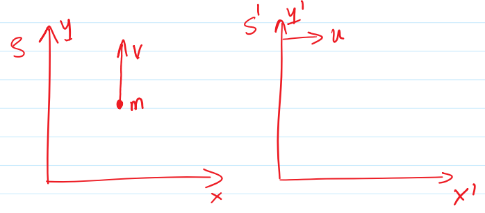
\(E=\gamma_v mc^2 , p_x=0\)
So, \(E'=\gamma_u(\gamma_v mc^2- 0)\)
\(E'=\gamma_u\gamma_v mc^2\)
Q.No:45 CSIR Sep-2022
If the average energy \(\langle E \rangle_T\) of a quantum harmonic oscillator at a temperature \(T\) is such that \(\langle E \rangle_T =2\langle E \rangle_{T\rightarrow 0}\), then \(T\) satisfies
(1)
\(coth \left( \frac{\hbar \omega}{k_B T} \right)=2\)
(2)
\(coth \left( \frac{\hbar \omega}{2k_B T} \right) =2\)
(3)
\(coth \left( \frac{\hbar \omega}{k_B T} \right) =4\)
(4)
\(coth\left( \frac{\hbar \omega}{2k_B T} \right) =4\)
Solution :
\(\epsilon_n=(n+\frac{1}{2}) \hbar \omega\)
\(z=\sum_n e^{-\beta \epsilon_n}=e^{-\beta\frac{\hbar}{2}\omega}+e^{-\beta\frac{3\hbar}{2}\omega}+e^{-\beta\frac{5\hbar}{2}\omega}+ ....\)
=\(e^{-\beta\frac{\hbar}{2}\omega}[1+e^{-\beta \hbar \omega}+e^{-2\beta \hbar \omega}+.....]\)
\(z=e^{-\beta\frac{\hbar}{2}\omega} \hspace{3mm} \frac{1}{1-e^{-\beta \hbar \omega}}\)
\(ln z = -\beta \frac{\hbar\omega}{2} - ln (1-e^{-\beta \hbar \omega})\)
\(\langle E\rangle=\frac{-\partial}{\partial \beta } \hspace{1mm}ln z= \frac{\hbar \omega}{2}+\frac{-e^{-\beta \hbar \omega}}{1-e^{-\beta \hbar \omega}}(-\hbar \omega)\)
\((\langle E\rangle)_T=\hbar \omega (\frac{1}{2}+\frac{1}{e^{\beta \hbar \omega}-1}), \hspace{5mm} \beta=\frac{1}{k_B T}\)
As \(T \to 0 \hspace{3mm}, \beta \to \infty, \hspace{3mm} e^{\beta \hbar \omega}\to \)large,
\((\langle E\rangle)_{T \to 0} \to \frac{\hbar \omega}{2}\) (Obviously)\\
(\(\langle E\rangle)_T=2(\langle E\rangle)_{T \to 0}\)
\(\hbar \omega (\frac{1}{2}+\frac{1}{e^{\beta \hbar \omega}-1})=\hbar \omega\)
\(\frac{1}{2}+\frac{1}{e^{\beta \hbar \omega}-1}=1\)
\(\frac{(e^{\beta \hbar \omega}-1)+2}{2(e^{\beta \hbar \omega}-1)}=1 \Rightarrow \frac{e^{\beta \hbar \omega}+1}{e^{\beta \hbar \omega}-1}=2\)
\(\frac{e^{\beta \frac{\hbar }{2}\omega}+{e^{-\beta \frac{\hbar }{2}\omega}}}{e^{\beta \frac{\hbar }{2}\omega}-{e^{-\beta \frac{\hbar }{2}\omega}}}=2\)
\(coth(\beta \frac{\hbar}{2}\omega)=2\)
\(coth(\frac{\hbar \omega}{2k_BT})=2\)
Q.No:46 CSIR Sep-2022
A high frequency voltage signal \(v_i=v_m sin \hspace{1mm}\omega t\) is applied to a parallel plate deflector as shown in the figure.

An electron beam is passing through the deflector along the central line. The best qualitative representation of the intensity \(I(t)\) of the beam after it goes through the narrow circular aperture \(D\), is


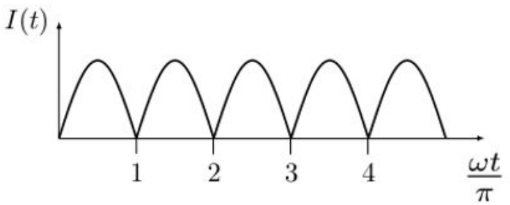
Solution :
When \(V_i\)=0 ( No changes on capacitor )

So, we will get high intensity every time \(V_i\) is zero.
\(V_i=V_m sin(\omega t)=0 \Rightarrow \omega t= n \pi\hspace{4mm} n=0,1,2,...\)
\(V_i=0\) when \(\frac{\omega t}{\pi}=n , \hspace{5mm} n=0,1,2,...\)

Q.No:47 CSIR Sep-2022
The Laplace transform \(L[f](y)\) of a function
\[ f(x)=
\begin{cases}
1, & 2n\leq x \leq 2n+1 \\
0, & 2n+1\leq x \leq 2n+2
\end{cases}
\]
n=0,1,2... is
(1)
\(\frac{e^{-y}(e^{-y}+1)}{y(e^{-2y}+1)}\)
(2)
\(\frac{e^{y}-e^{-y}}{y}\)
(3)
\(\frac{e^{y}+e^{-y}}{y}\)
(4)
\(\frac{e^{y}(e^{y}-1)}{y(e^{2y}-1)}\)
Solution :
\(L[f]y=\int_0 ^\infty f(x) \cdot e^{-yx}dx\)
When \(n=0\)
\(f(x)=\begin{cases}
1, & 0\leq x \leq 1 \\
0, & 1\leq x \leq 2
\end{cases}\)
When \(n=1\)
\(f(x)=\begin{cases}
1, & 2\leq x \leq 3 \\
0, & 3\leq x \leq 4
\end{cases}\)
and so on
\(L[f](y)=\int_0^1 1 \cdot e^{-yx}dx +\int_2^3 1 \cdot e^{-yx}dx+ \int_4 ^ 5 1 \cdot e^{-yx}dx + ....... \)
=\(-\frac{1}{y}[e^{-yx}]_0^1-\frac{1}{y}[e^{-yx}]_2^3-\frac{1}{y}[e^{-yx}]_4 ^5+......]\)
=\(-\frac{1}{y}[(e^{-y}-1)+(e^{-3y}-e^{-2y})+(e^{-5y}-e^{-4y})+........]\)
=\(\frac{1}{y}[1-e^{-y}+e^{-2y}-e^{-3y}+e^{-4y}-e^{-5y}+.......]\)
=\(\frac{1}{y} [(1+e^{-2y}+e^{-4y}+....) -(e^{-y}+e^{-3y}+e^{-5y}+......)]\)
=\(\frac{1}{y}[\frac{1}{(1-e^{-2y})}-e^{-y}(\frac{1}{1-e^{-2y}})]\)
=\(\frac{1}{y}\frac{(1-e^{-y})}{(1-e^{-2y})}=\frac{1}{y}\frac{e^{-y}(e^{y}-1)}{e^{-2y}(e^{2y}-1)}=\frac{1}{y}\frac{e^y(e^y-1)}{(e^{2y}-1)}\)
Q.No:48 CSIR Sep-2022
The electronic configuration of \(^{12}C\) is \(1s^2, 2s^2, 2p^2\). Including LS coupling, the correct ordering of it's energy is
(1)
\(E(^3P_2)<E(^3P_1)<E(^3P_0)<E(^1D_2)\),
(2)
\(E(^3P_0)<E(^3P_1)<E(^3P_2)<E(^1D_2)\),
(3)
\(E(^1D_2)<E(^3P_2)<E(^3P_1)<E(^3P_0)\),
(4)
\(E(^3P_1)<E(^3P_0)<E(^3P_2)<E(^1D_2)\),
Solution :
There are two equivalent electrons in p orbit. It is less than half filled.
According to Hund's rule :
(1) The highest total spin (S) state have the lowest energy.
(2) For a given spin (S), the highest total \(L\) state have the lowest energy
(3) For a given \(L\) and \(S\) and for less than half filled, lower \(J\) value state will be lie below.
Summary: Singlets are always above the triplets. Within multiplicity, and within \(L\), lower \(J\) value state lie below for less than half filled orbits.
So, \(E(^3P)< E(^1D)\)
\(E(^3 P_0)<E(^3 P_1)<E(^3 P_2)< E(^1 D_2)\)
Q.No:50 CSIR Sep-2022
To first order in perturbation theory, the energy of the ground state of the Hamiltonian
\[
H=\frac{p^2}{2m} + \frac{1}{2} m \omega^2 x^2
+ \frac{\hbar \omega}{\sqrt{512}}exp\left[-\frac{m\omega}{\hbar}x^2\right]
\]
(1)
\(\frac{15}{32}\hbar \omega\)
(2)
\(\frac{17}{32}\hbar \omega\)
(3)
\(\frac{19}{32}\hbar \omega\)
(4)
\(\frac{21}{32}\hbar \omega\)
Solution :
\(H'=\frac{\hbar \omega}{\sqrt{512}}\)exp \([-\frac{m \omega}{\hbar}x^2]\hspace{6mm} \psi_0=(\frac{m\omega}{\pi \hbar})^{1/4} e^{-\frac{m \omega}{2\pi}x^2}\)
According to perturbation theory, first order correction to ground state is \(E_0 ^{(1)}=\langle \psi_0| H' |\psi_0\rangle\)
\(E_0 ^{(1)}=\sqrt{\frac{m \omega}{\pi \hbar}} \frac{\hbar \omega}{\sqrt{512}}\int_{-\infty}^{+\infty}e^{\frac{-2m \omega}{\hbar}x^2}dx = \frac{\hbar \omega}{\sqrt{512 \times 2}}=\frac{\hbar \omega}{32}\)
Energy up to first order :
\(E_0^{(0)}+E_0^{(1)}=\frac{\hbar \omega}{2}+\frac{\hbar \omega}{32}=\frac{17}{32}\hbar \omega\)
Q.No:52 CSIR Sep-2022
A bucket contains 6 red and 4 blue balls. A ball is taken out of the bucket at random and two balls of the same colour are put back. This step is repeated once more. The probability that the numbers of red and blue balls are equal at the end, is
(1)
4/11
(2)
2/11
(3)
1/4
(4)
3/4
Solution :
When will you end up with same number of red and blue ball ?

Step(1): A blue ball is taken out of the bucket containing 6 red and 4 blue balls.
Two blue balls are put back. Now bucket contains 6 red and 5 blue balls.
Step(2): Then, one more blue ball is taken out again from the bucket containing 6 red and 5 blue balls.
Two blue balls are put back.
Now bucket contain 6 red and 6 blue balls.
Probability of picking a blue ball in Step(1)=\(\frac{4}{10}\)
Probability of picking a blue ball in Step (2)=\(\frac{5}{11}\)
Total probability=\(\frac{4}{10} \times \frac{5}{11}=\frac{2}{11}\)
Q.No:53 CSIR Sep-2022
In the absorption spectrum of H-atom, the frequency of transition from the ground state to the first excited state is \(\nu_H\). The corresponding frequency for a bound state of a positively charged muon \(\mu^+\) and an electron is \(\nu_\mu\). Using \(m_\mu=10^{-28}kg\), \(m_e=10^{-30}kg\) and \(m_p>>m_e,m_\mu\), the value of
\((\nu_\mu -\nu_H)/\nu_H\) is
(1)
0.001
(2)
–0.001
(3)
-0.01
(4)
0.01
Solution :
Since the transmission are between the same levels, frequency is proportional to Rydberg constant.
Rydberg constant \(\propto \) reduced mass (Need to remember)
For H-atom, reduced mass \(\simeq m_e\)
For \(\mu^+\) and electron reduced mass =\(\frac{m_e \times m_{\mu}}{m_e+m_{\mu}}=\frac{m_e}{\frac{m_e}{m_{\mu}}+1}
=0.99m_e\)
So,
\[
\frac{\nu_\mu - \nu_H}{\nu_\mu} = 1 - \frac{\nu_H}{\nu_\mu} = 1 - \frac{R_H}{R_\mu} = 1- \frac{m_e}{0.99 m_e} = 1-1.010 =-0.01
\]
Q.No:56 CSIR Sep-2022
A paramagnetic salt with magnetic moment per ion \(\mu_\pm=\pm \mu_B\) (where \(\mu_B\) is the Bohr magneton) is in thermal equilibrium at temperature \(T\) in a constant magnetic field \(B\). The average magnetic moment \(\langle M \rangle\), as a function of \(k_BT/\mu_BB\) is best represented by


Solution :
Possible energies \(\epsilon =\pm \mu_B B\)
Partition function \[z=e^{-\beta\mu_B B}+e^{+\beta\mu_B B} = 2 \hspace{2mm} cosh(\beta \mu_B B)\]
Average energy
\[\langle E \rangle =\frac{-\partial}{\partial \beta}ln (z)=-\mu_B B \hspace{2mm} tanh(\beta \mu_B B)\]
\[\langle M \rangle= -\langle E \rangle/B = \mu_B \hspace{2mm} tanh(\frac{\mu_B B}{k_B T})\]
\(\langle M \rangle\) is plotted v/s \(\frac{k_B T}{\mu_B B}\)
Taking \(\langle M \rangle=y\) and \(\frac{k_B T}{\mu_B B}=x\)
\[\langle M \rangle=y= \mu_B tanh (\frac{1}{x})\]
as \(x\to 0, \frac{1}{x}\to \)large , tanh\((\frac{1}{x})\to 1\)
as \(x\to \infty, \frac{1}{x}\to \)small , tanh\((\frac{1}{x})\to \frac{1}{x}\)
as \(x\to 0 \hspace{2mm} \langle M \rangle \to \mu_0\)
as \(x\to \infty \hspace{2mm} \langle M \rangle \to \mu_0\frac{1}{x}\)
Option 3 is the approximate representation.
Q.No:57
The energy/energies \(E\) of the bound state(s) of a particle of mass \(m\) in one dimension in the potential
\[
V(x)= \begin{cases}
\infty, & x \leq 0 \\
-V_0, & 0 \le x \le a \\
0, & x \geq a
\end{cases}
\]
(1) \(cot^2\left( a \sqrt{\frac{2m(E+V_0)}{\hbar^2}}\right) = \frac{E-V_0}{E}\)
(2) \(tan^2\left( a \sqrt{\frac{2m(E+V_0)}{\hbar^2}}\right) =-\frac{E}{E+V_0}\)
(3) \(cot^2\left( a \sqrt{\frac{2m(E+V_0)}{\hbar^2}}\right) =-\frac{E}{E+V_0}\)
(4) \(tan^2\left( a \sqrt{\frac{2m(E+V_0)}{\hbar^2}}\right) = \frac{E-V_0}{E}\)
Solution :
Refer Zettili Problem 4.13, outside 4th Chapter. This is a solved problem in Zettili.
For bound state, energy E<0. Wave function vanishes for Region-1, as potential is infinite there. It is sinusoidal for Region-2, which is classically allowed region. For Region-3, classically forbidden region, it is exponentially decaying.

For Region-2, \(E>V\), \(V=-V_0\)
\[
k= \frac{\sqrt{2m(E-V)}}{\hbar} = \frac{\sqrt{2m(E+V_0)}}{\hbar}
\]
For Region-3, \(E<V\), \(V=0\),
\[
\kappa = \frac{\sqrt{2m(V-E)}}{\hbar} = \frac{\sqrt{-2mE}}{\hbar}
\]
Continuity of the wave function at \(x=0\), leads to
\[\psi_1(0)=\psi_2(0)\]
\[0=A \cdot 0 + B \cdot 1 \Rightarrow B=0\]
So, the wave-function in Region-2 becomes
\[\psi_2(x)=A \hspace{1mm}sin(kx) \]
(Don't apply derivative continuity at x=0, because derivative is discontinuous at x=0 as potential touching infinity )
Continuity of the wave function and it's derivative at \(x=a\), leads to
\[
\psi_2(a)=\psi_3(a) \Rightarrow A \hspace{1mm} sin(ka)=Ce^{-\kappa a} \hspace{3mm}---(I)
\]
\[
\psi'_2(a)=\psi'_3(a) \Rightarrow A \hspace{1mm}k \hspace{1mm} cos(ka)=-C \kappa e^{-\kappa a} \hspace{3mm}---(II)
\]
(II)/(I) leads to
\[
k \hspace{1mm} cot(ka) = -\kappa
\]
\[
cot^2(ka)= \frac{\kappa^2}{k^2}
\]
Substituting \(k\) and \(\kappa\) from above relations, we get
\[
cot^2\left(\frac{\sqrt{2m(E+V_0)}}{\hbar}a\right) = -\frac{E}{E+V_0}
\]
Q.No: 60
The Lagrangian of a system of two particles is
\[
L= \frac{1}{2} \dot{x_1}^2 + 2
\dot{x_2}^2 - \frac{1}{2}
(x_1^2 + x_2^2 + x_1 x_2)\]
The normal frequencies are best approximated by
(1) 1.2 and 0.7
(2) 1.5 and 0.5
(3) 1.7 and 0.5
(4) 1.0 and 0.4
Solution :
Kinetic Energy :
\[
T=\frac{1}{2} (\dot{x_1}^2 + 4
\dot{x_2}^2)
\]
Potential Energy :
\[
V(x)=\frac{1}{2}
\left[x_1^2 + x_2^2 + \frac{1}{2}(x_1 x_2) + \frac{1}{2}(x_2 x_1) \right]
\]
T and V matrices are (apart from 1/2 factor taken outside in the above equations)
\[
T= \begin{pmatrix}
1&0\\
0&4
\end{pmatrix}, \hspace{2mm}
V= \begin{pmatrix}
1&1/2\\
1/2&1
\end{pmatrix}
\]
To find normal mode frequencies, we need to solve this determinant for \(\omega\)
\[
|V-\omega^2T|=0
\]
\[
\begin{vmatrix}
1-\omega^2 & 1/2 \\
1/2 & 1-4\omega^2
\end{vmatrix} =0
\]
After solving this determinant for \(\omega^2\), we get
\[
\omega^2 = \frac{20 \pm 14.42}{32}
\]
(Calculator is needed).
So, two normal mode frequencies are
\[
\omega_1= 0.41, \hspace{2mm} \omega_2=1.037
\]
Option 4 would be an appropriate one.
Q.No:60 CSIR Sep-2022
Two parallel conducting rings, both of radius \(R\), are separated by a distance \(R\). The planes of the rings are perpendicular to the line joining their centers, which is taken to be \(x\)-axis.

If both the rings carry the same current \(i\) along the same direction, the magnitude of the magnetic field along \(x-\)axis is best represented by


Solution :
This is the famous Helmholtz Coil used for producing a region of nearly uniform magnetic field.
(Refer Problem 5.46 Griffiths Electrodynamics 4th edition)
When distance between rings = \(R\), \(\frac{\partial B}{\partial x}=0\) and \(\frac{\partial^2 B}{\partial x^2}=0\),
which leads to uniform magnetic field at the center region. At this condition, magnetic fields at the planes of coil are little bit smaller than that at the center.
So, Option 1 is an approximate diagram.
Q.No:61
At time \(t=0\), a particle in the ground state of the Hamiltonian
\[
H(t)=\frac{p^2}{2m} + \frac{1}{2} m \omega^2 x^2
+ \lambda x sin(\frac{\omega t}{2} )\]
where \(\lambda\) \(\omega\) and \(m\) are positive constants. To \(O(\lambda^2)\), the probability that at \(t=2\pi/\omega\), the particle would be in the first excited state of \(H(t=0)\) is
(1) \(\frac{9 \lambda^2}{16 m \hbar \omega^3}\)
(2) \(\frac{9 \lambda^2}{8 m \hbar \omega^3}\)
(3) \(\frac{16 \lambda^2}{9 m \hbar \omega^3}\)
(4) \(\frac{8 \lambda^2}{9 m \hbar \omega^3}\)
Solution :
Consider two states \(\psi_a\) and \(\psi_b\) with respective energies \(E_a\) and \(E_b\). We define \(\omega_0=(E_b-E_a)/\hbar\).
When there exist Time-Dependent Perturbation \(H'(t)\), Probability of transition \(P_{a \rightarrow b}(t) = |c_b(t)|^2\), where
\[
c_b(t) = -\frac{i}{\hbar} \int_0^t H'_{ab}(t') e^{i\omega_0 t'} dt'
\]
Where \(H'_{ab}(t') = \langle \psi_a | H'(t) |\psi_b \rangle \)
In the present problem, \(H'(t)= \lambda x \hspace{1mm} sin(\omega t/2)\)
\[
\psi_a = \psi_0 = \left(\frac{m\omega}{\pi \hbar}\right)^{1/4} e^{-\frac{m \omega}{2\pi}x^2}
\]
\[
\psi_b = \psi_1 = \left(\frac{m\omega}{\pi \hbar}\right)^{1/4} \sqrt{\frac{2m\omega}{\hbar}} x e^{-\frac{m \omega}{2\pi}x^2}
\]
\[
H'_{ab}=H'_{01}= \int_{-\infty}^{+\infty} \psi_a^* H'(t) \psi_b dx = \lambda \sqrt{\frac{\hbar}{2m\omega}} sin(\omega t/2)
\]
Use the following integral
\[
\int_{0}^{+\infty} x^n e^{-ax^2} dx
= \frac{1}{2a^{(n+1)/2}} \Gamma \left[(n+1)/2\right]\]
With \( \Gamma(1/2)=\sqrt{\pi}\)
In this case, \(\omega_0 = (E_1-E_0)/\hbar = \omega\)As we need Probability at \(t=2\pi/\omega\), \[
c_1(2\pi/\omega) = -\frac{i}{\hbar} \int_0^{2\pi/\omega} H'_{01}(t') e^{i\omega_0 t'} dt'
\]
\[
c_1(2\pi/\omega) = -\frac{i}{\hbar} \lambda \sqrt{\frac{\hbar}{2m\omega}} \int_0^{2\pi/\omega} sin(\omega t/2) e^{i\omega t} dt
\]
\[
c_1(2\pi/\omega) = -\frac{\lambda}{\hbar} \sqrt{\frac{\hbar}{2m\omega}} \frac{1}{i\omega} \frac{4}{3}
\]
So, probability at \(t=2\pi/\omega\)
\[
P_{0 \rightarrow 1}(2\pi/\omega)= |c_1(2\pi/\omega)|^2 = \frac{8 \lambda^2}{9m\hbar \omega^3}
\]
Q.No:62 CSIR Sep-2022
The energies of two level system are \(\pm E\). Consider an ensemble of such non interacting systems at temperature \(T\). At low temperatures, the leading term in the specific heat depend on T as
(1)
\(\frac{1}{T^2} e^{-E/k_BT}\)
(2)
\(\frac{1}{T^2} e^{-2E/k_BT}\)
(3)
\(T^2 e^{-E/k_BT}\)
(4)
\(T^2 e^{-2E/k_BT}\)
Solution :
Partition function \(z=e^{-\beta E}+e^{+\beta E}= 2 \hspace{2mm} cosh (\beta E)\)
\[\bar{E}=\frac{-\partial}{\partial \beta}ln \hspace{2mm}z=-E\hspace{2mm} tan h(\beta E) \]
\[C_v=-\frac{1}{k_B T^2}\frac{\partial}{\partial \beta}(\bar{E})=\frac{E}{k_B T^2} \hspace{4mm} sech^2(\beta E)\]
\[sech^2(\beta E)=\frac{1}{cosh^2(\beta E)}=\frac{4}{(e^{\beta E}+e^{-\beta E})^2}\]
At low temperature, \(\beta \to \) high, \(e^{-\beta E}\) is low,
\[e^{\beta E}+e^{-\beta E} \simeq e^{\beta E}, \hspace{3mm}sech^2(\beta E)\simeq 4 \hspace{2mm}e^{-2 \beta E}\]
\[C_v\propto \frac{1}{T^2}e^{-2 \beta E}\]
Q.No:63 CSIR Sep-2022
A system of N non-interacting particles in one-dimension, each of which is in a potential \(V(x)=gx^6\) where \(g>0\) is a constant and \(x\) denotes the displacement of the particle from its equilibrium position. In thermal equilibrium, the heat capacity at constant volume is
(1)
\(\frac{7}{6}Nk_B\)
(2)
\(\frac{4}{3}Nk_B\)
(3)
\(\frac{3}{2}Nk_B\)
(4)
\(\frac{2}{3}Nk_B\)
Solution :
\(V(x)= g \hspace{1mm} x^6\)
\[E=\frac{P_x^2}{2m} +g \hspace{1mm} x^6\]
\[\langle E \rangle =\langle \frac{p_x^2}{2m} \rangle +\langle g \hspace{1mm} x^6 \rangle\]
\[\langle \frac{p_x^2}{2m} \rangle=\frac{1}{2} k_B T \hspace{ 2mm}( Equi-partition \hspace{2mm} theorem)\]
\[\langle g \hspace{1mm} x^6 \rangle=\frac{\int_{-\infty} ^{+\infty}g \hspace{1mm} x^6 e^{-\beta g \hspace{1mm} x^6}dx}{\int_{-\infty} ^{+\infty}e^{-\beta g x^6}dx}
=
-\frac{\frac{d}{d \beta }\int_{-\infty} ^{+\infty}e^{-\beta g x^6}dx} {\int_{-\infty} ^{+\infty}e^{-\beta g x^6}dx}\]
\[= -\frac{d}{d \beta} \left[ln \hspace{2mm} \left(\int_{-\infty} ^{+\infty}e^{-\beta g x^6}dx\right)\right]\]
\[I=\int_{-\infty} ^{+\infty}e^{-\beta g x^6}dx =2\int_{0} ^{+\infty}e^{-\beta g x^6}dx\]
\[\int_{0} ^{+\infty} e^{-Ax^n} dx =\frac{1}{nA^{1/n}}\Gamma (\frac{1}{n})\]
\[I=2\frac{1}{(\beta g)^{\frac{1}{6}}}\Gamma(\frac{1}{6})\]
\[\langle g \hspace{1mm} x^6 \rangle=-\frac{d}{d \beta}[ln \hspace{1mm} C_1-\frac{1}{6}ln \hspace{1mm} \beta] = \frac{1}{6}\hspace{1mm}\frac{1}{\beta}=\frac{1}{6} k_B T\]
\[\langle E \rangle =\frac{k_B T}{2}+\frac{k_B T}{6}=\frac{2k_B T}{3}\]
Average energy for \(N\) particles
\(\langle E \rangle=\frac{2}{3}NK_B T\)
Specific heat :
\(C_v=\frac{\partial \langle E \rangle}{\partial T}= \frac{2}{3}NK_B\)
Q.No:64 CSIR Sep-2022
The Hamiltonian of a spin-1/2 particle in a magnetic field \(\textbf{B}=B_0 \hat{\textbf{k}}\) is given by \(H=\lambda \textbf{S} \cdot \textbf{B}\), where \(\textbf{S}\) is its spin (in units of \(\hbar\)) and \(\lambda \) is constant. If the average spin density is \( \langle \textbf{S} \rangle\) for an ensemble of such non-interacting particles, then \(\frac{d}{dt} \langle S_x \rangle \) is
(1)
\(\frac{\lambda}{\hbar} B_0 \langle S_x \rangle \)
(2)
\(\frac{\lambda}{\hbar} B_0 \langle S_y \rangle \)
(3)
\(-\frac{\lambda}{\hbar} B_0 \langle S_x \rangle \)
(4)
\(-\frac{\lambda}{\hbar} B_0 \langle S_y \rangle \)
Solution :
\(H=\lambda B_0 S_z\)
\[
\frac{d}{dt}\langle S_x \rangle = \frac{1}{i\hbar} \langle [S_x, H] \rangle + \langle \frac{\partial S_x}{\partial t} \rangle
\]
\[
[S_x, H] = [S_x, \lambda B_0 S_z] = \lambda B_0 [S_x, S_z] = \lambda B_0 (-i\hbar S_y)
\]
\[
\frac{\partial S_x}{\partial t} =0 \hspace{2mm} (In \hspace{2mm} Schrodinger \hspace{2mm} picture)
\]
\[
\frac{d}{dt}\langle S_x \rangle = -\lambda B_0 \langle S_y \rangle
\]
It is mentioned in the question that spin is defined in the units of \(\hbar\). Hence answer is Option: 4
Q.No:67 CSIR Sep-2022
Two small metallic objects are embedded in a weakly conducting medium of conductivity \(\sigma\), and dielectric constant \(\epsilon\). A battery connected between them leads to a potential difference \(V_0\). It is subsequently disconnected at time \(t=0\). The potential difference at later time \(t\) is
(1)
\(V_0 e^{-t\sigma/4\epsilon}\)
(2)
\(V_0 e^{-t\sigma/2\epsilon}\)
(3)
\(V_0 e^{-3t\sigma/4\epsilon}\)
(4)
\(V_0 e^{-t\sigma/\epsilon}\)
Solution :
Refer Problem 7.3 Griffiths Electrodynamics 4th Edition. Capacitance (C) of the configuration is related to resistance (R) and conductivity (\(\sigma\)) by the relation :
\[
C=\frac{\epsilon}{\sigma R}
\]

\[
V(t) = V_0 e^{-t/RC} = V_0 e^{-t \sigma/\epsilon}
\]
Q.No:68 CSIR Sep-2022
The value of the integral
\[\int_{-\infty}^{\infty} \frac{\cos{(ax)}}{x^2+1} dx
\]
for \(a > 0 \)
(1)
\(\pi e^\alpha\)
(2)
\(\pi e^{-\alpha}\)
(3)
\(\pi e^{-\alpha/2}\)
(4)
\(\pi e^{\alpha/2}\)
Solution :
\[I=\int_{-\infty} ^{+\infty} \frac{cos(ax)}{x^2 + 1} dx = Re \left ( \int_{-\infty} ^{+\infty} \frac{e^{iax}}{x^2 + 1} dx \right)\]
To solve \(\int_{-\infty} ^{+\infty} \frac{e^{iax}}{x^2 + 1} dx\) for \(a>0\), we need to choose semi-circular contour in the upper half plane (Followed by Weber).
Consider contour integral of \(\frac{e^{iaz}}{z^2 + 1} dz\) around this semi-circular contour

\[
\oint \frac{e^{iaz}}{z^2 + 1} dz =\int_{curved} \frac{e^{iaz}}{z^2 + 1} + \int_{-R} ^{+R} \frac{e^{iax}}{x^2 + 1} dx
\]
As \(R \Rightarrow \infty\), curved part of contour integral vanishes, and the limit of integral on real axis becomes \(-\infty \Rightarrow +\infty\). Contour covers entire upper half plane.
\[
\oint \frac{e^{iaz}}{z^2 + 1} dz = \int_{-\infty} ^{+\infty} \frac{e^{iax}}{x^2 + 1} dx
\]
\[
= 2\pi i \times Residue \hspace{2mm} of \frac{e^{iaz}}{z^2 + 1} \hspace{2mm} in \hspace{2mm}upper \hspace{2mm} half \hspace{2mm} plane
\]
\(z=i\) is only singularity in upper half plane. So, residue at \(z=i\)
\[
R(z=i) = \lim_{z \to i} (z-i) \frac{e^{iaz}}{(z-i)(z+i)} = \frac{e^{-a}}{2i}
\]
\[\int_{-\infty} ^{+\infty} \frac{e^{iax}}{x^2 + 1} dx = \pi e^{-a}
\]
So, the given integral which is real part of above integral is \(\pi e^{-a}\).
Answer : 2
Q.No:70 CSIR Sep-2022
A square conducting loop in \(yz\)-plane, falls downward under the gravity along the negaive \(z\)-axis. Region1, defined by \(z>0\) has a uniform magnetic field \(\textbf{B}=B_0 \hat{\textbf{i}}\), while region 2 (defined by \(z<0\)) has no magnetic field.


Solution :
When the conducting loop falling in the Region-1, there will be no rate of change of flux, no net magnetic force and hence no induced EMF. So, there will be no opposition to the motion (No Lenz law). So, it is a constant accelerated motion (a=g).
When it falling in Region-2 where there is no magnetic field, again it is a constant accelerated motion.

During the time when the loop enters Region-2 from Region-1 and being partially in Region-1 and Region-2, and falling, the flux is decreasing. EMF will be induced in the loop to produce the current in anti-clockwise direction (According to Lenz law). Now, upper portion of the current carrying loop which is still in magnetic field experience magnetic force \(\vec{F}= \int (\vec{I} \times \vec{B}) dl\) in the upward direction resulting decrease of net downward force and hence acceleration.
As we know, slope of v-t graph is acceleration, and in Option-2, slope was a constant and was decreasing and then constant as earlier.
Q.No:71 CSIR Sep-2022
The matrix corresponds to differential operator \((1+\frac{d}{dx})\) in the space of polynomial of degree at most two in the basis spanned by \(f_1=1\), \(f_2=x\) and \(f_3=x^2\), is
(1)
\(
\begin{pmatrix}
1 & 1 & 0 \\
0 & 1 & 2 \\
0 & 0 & 1
\end{pmatrix}
\)
(2)
\(
\begin{pmatrix}
1 & 0 & 0 \\
1 & 1 & 0 \\
0 & 2 & 1
\end{pmatrix}
\)
(3)
\(
\begin{pmatrix}
1 & 1 & 0 \\
0 & 1 & 1 \\
0 & 0 & 2
\end{pmatrix}
\)
(4)
\(
\begin{pmatrix}
1 & 0 & 0 \\
1 & 1 & 0 \\
0 & 1 & 2
\end{pmatrix}
\)
Solution :
Basis : \(\{|f_1\rangle=1, |f_2\rangle=x, |f_3\rangle=x^2 \} \)
Let us take the simplest vector in this basis
\[
|\psi \rangle = 1+x+x^2 = |f_1\rangle + |f_2\rangle + |f_3\rangle = \begin{pmatrix} 1\\1\\1 \end{pmatrix}
\]
Let \(\hat{Q} = 1+d/dx\)
\[
\hat{Q}|\psi \rangle = \left(1 + \frac{d}{dx}\right) [1+x+x^2] = 2 + 3x + x^2
\]
\[
\hat{Q}|\psi \rangle = |\phi \rangle = 2 + 3x + x^2 = 2|f_1\rangle + 3|f_2\rangle + 1|f_3\rangle = \begin{pmatrix} 2\\3\\1 \end{pmatrix}
\]
\[
Q_{3\times3} \begin{pmatrix} 1\\1\\1 \end{pmatrix} = \begin{pmatrix} 2\\3\\1 \end{pmatrix}
\] (In this basis).
Among the options, find the matrix Q which satisfy above relation.
OR
If \(|\psi\rangle= c_1|f_1\rangle + c_2|f_2\rangle + c_3|f_3\rangle\), then
\(\hat{Q}|\psi\rangle= |\phi \rangle = c'_1|f_1\rangle + c'_2|f_2\rangle + c'_3|f_3\rangle\)
In matrix form,
\[
Q_{3\times3} \cdot \begin{pmatrix} c_1\\c_2\\c_3 \end{pmatrix} = \begin{pmatrix} c'_1\\c'_2\\c'_3 \end{pmatrix}
\]
\[
\hat{Q}|f_1 \rangle = 1= 1|f_1\rangle + 0|f_2\rangle + 0|f_3\rangle
\]
\[
\hat{Q}|f_2 \rangle = 1+x = 1|f_1\rangle + 1|f_2\rangle + 0|f_3\rangle
\]
\[
\hat{Q}|f_3 \rangle = 2x + x^2 = 0|f_1\rangle + 2|f_2\rangle + 1|f_3\rangle
\]
\(\hat{Q}|\psi\rangle=c_1\hat{Q}|f_1\rangle + c_2\hat{Q}|f_2\rangle + c_3\hat{Q}|f_3\rangle \\ = c_1|f_1\rangle + c_2(|f_1\rangle + |f_2\rangle) + c_3(2|f_2\rangle+ 1|f_3\rangle) \\
= (c_1+c_2)|f_1\rangle + (c_2+2c_3)|f_2\rangle + c_3|f_3\rangle \\
= c'_1|f_1\rangle + c'_2|f_2\rangle + c'_3|f_3\rangle
\)
\(c'_1=1c_1+1c_2+0c_3\)
\(c'_2=0c_1+1c_2+2c_3\)
\(c'_3=0c_1+0c_2+1c_3\)
\[
\begin{pmatrix} c'_1\\c'_2\\c'_3 \end{pmatrix} = \begin{pmatrix} 1&1&0\\
0&1&2\\
0&0&1\end{pmatrix} \cdot \begin{pmatrix} c_1\\c_2\\c_3 \end{pmatrix}
\]
Answer : 1
Q.No:72 CSIR Sep-2022
A stationary magnetic dipole \(\textbf{m}=m\hat{\textbf{k}}\) is placed above an infinite surface (\(z=0\)) carrying uniform surface current density \(\vec{\kappa}\)=\(\kappa\hat{\textbf{i}}\).
The torque on the dipole is
(1)
\(\frac{\mu_0}{2} m \kappa \hat{\textbf{i}} \)
(2)
\(-\frac{\mu_0}{2} m \kappa\hat{\textbf{i}} \)
(3)
\(\frac{\mu_0}{2} m \kappa \hat{\textbf{j}}\)
(4)
\(-\frac{\mu_0}{2} m \kappa \hat{\textbf{j}}\)
Solution :
\(\vec{m}=m\hat{k}\)

\(\vec{B}_{above}=\frac{\mu_0 k}{2}(-\hat{j})\)
Torque \(\vec{N}=\vec{m} \times \vec{B}= m\hat{k}\times \frac{\mu_0 k}{2}(-\hat{j})\)
\(\vec{N}=\frac{m \mu_0 k}{2}\hat{i}\)
Q.No:74 CSIR Sep-2022
The energy levels of a system, which is in equilibrium at temperature \(T=1/k_B \beta\), are 0, \(\epsilon\), and \(2\epsilon\). If two identical bosons occupy these energy levels, the probability of the total energy being \(3\epsilon\) is
(1)
\(\frac{e^{-3\beta\epsilon}}{1+e^{-\beta\epsilon}+e^{-2\beta\epsilon}+e^{-3\beta\epsilon}+e^{-4\beta\epsilon}}\)
(2)
\(\frac{e^{-3\beta\epsilon}}{1+2e^{-\beta\epsilon}+2e^{-2\beta\epsilon}+e^{-3\beta\epsilon}+e^{-4\beta\epsilon}}\)
(3)
\(\frac{e^{-3\beta\epsilon}}{e^{-\beta\epsilon}+2e^{-2\beta\epsilon}+e^{-3\beta\epsilon}+e^{-4\beta\epsilon}}\)
(4)
\(\frac{e^{-3\beta\epsilon}}{1+e^{-\beta\epsilon}+2e^{-2\beta\epsilon}+e^{-3\beta\epsilon}+e^{-4\beta\epsilon}}\)
Solution :
Distributing two identical bosons in three levels

Partition function
\(Z=\sum_R e^{-\beta E_R}=1+ e^{-\beta \epsilon }+2e^{-2\beta \epsilon }+e^{-3\beta \epsilon }+e^{-4\beta \epsilon }\)
There is only one way of getting energy \(3\epsilon\)
So, \(P(3\epsilon)=\frac{e^{-3\beta \epsilon }}{Z}\)
Q.No:75 CSIR Sep-2022
The Lagrangian of a particle n one dimension is
\[
L=\frac{m}{2} \dot{x}^2-ax^2-V_0 e^{-10x}
\]
where \(a\) and \(V_0\) are positive constants. The best qualitative representation of a trajectory in phase space is


Solution :
Corresponding Hamiltonian
\[H=\frac{P_x ^2}{2m}+ax^2+V_0e^{-10x} \]
For a particular energy :
\[E=\frac{P^2}{2m}+ax^2+V_0e^{-10x}\]
This is not elliptical relation between \(p\) and \(x\). So, we can eliminate option 3 and 4.
Potential energy \(V(x)=ax^2+V_0e^{-10x}\) has its minimum at \(x>0\) (Go for derivative test). When we decrease energy, phase space closed curve shrinks at potential minimum ( stable equilibrium )
Refer to this video link : https://youtu.be/N42tp-_Fn04
Option 1 is shrinks at \(x_0 < 0\)
Option 2 is shrinks at \(x_0 > 0\)

So, Option 2 is appropriate .
For accurate analysis, plot \(V(x)\) properly and follow our trick explained in the above video.